Numpy Tutorials 02 [Notion : 1/9]

Numpy Tutorials

• Numpy is the core library for scientific computing in Python.
• Ref link : https://cs231n.github.io/python-numpy-tutorial/

# Module Import
import numpy as np

Boolean array indexing

Boolean array indexing lets you pick out arbitrary elements of an array.
Frequently this type of indexing is used to select the elements of an array that satisfy some condition.

a = np.array([1,2],[3,4],[5,6])
bool_idx = (a > 2) # Find the elements of a that are bigger than 2
				   # this returns a numpy array of Booleans of the same
				   # shape as a, where each slot of bool_idx tells
				   # whether that element of a in > 2.
print(bool_idx)
# [[False False],
#  [True   True],
#  [True   True]]

# We use boolean array indexing to construct a rank 1 array
# consisting of the elements of a corresponding to the True values
# of bool_idx
print(a[bool_idx]) # [3,4,5,6]

# We can do all of the above in a single concise statement:
print(a[a>2]) # [3,4,5,6]

Datatypes

Every numpy array is a grid of elements of the same type.
Numpy provides a large set of numeric datatypes that you can use to construct arrays.
Numpy tries to guess a datatype when you create an array, but functions that construct arrays usually also include an optional argument to explicitly specify the datatype.

x = np.array([1,2])
print(x.dtype) # int64

x = np.array([1.0, 2.0])
print(x.dtype) # float64

x = np.array([1,2], dtype=np.int64)
print(x.dtype) # int64

Array math

Basic mathematical functions operate elementwise on arrays, and are available both as operator overloads and as functions in the numpy module

x = np.array([[1,2],[3,4]], dtype=np.float64)
y = np.array([[5,6],[7,8]], dtype=np.float64)

# Elementwise sum; both produce the array
# [[ 6.0  8.0]
#  [10.0 12.0]]
print(x + y)
print(np.add(x, y))

# Elementwise difference; both produce the array
# [[-4.0 -4.0]
#  [-4.0 -4.0]]
print(x - y)
print(np.subtract(x, y))

# Elementwise product; both produce the array
# [[ 5.0 12.0]
#  [21.0 32.0]]
print(x * y)
print(np.multiply(x, y))

# Elementwise division; both produce the array
# [[ 0.2         0.33333333]
#  [ 0.42857143  0.5       ]]
print(x / y)
print(np.divide(x, y))

# Elementwise square root; produces the array
# [[ 1.          1.41421356]
#  [ 1.73205081  2.        ]]
print(np.sqrt(x))

* is elementwise multiplication, not matrix multiplication.
We instead use the dot function to compute inner products of vectors, to multiply a vector by a matrix, and to multiply matrices. dot is available both as a function in the numpy module and as an instance method of array objects

x = np.array([[1,2],[3,4]])
y = np.array([[5,6],[7,8]])

v = np.array([9,10])
w = np.array([11, 12])

# Inner product of vectors; both produce 219
print(v.dot(w))
print(np.dot(v, w))

# Matrix / vector product; both produce the rank 1 array [29 67]
print(x.dot(v))
print(np.dot(x, v))

# Matrix / matrix product; both produce the rank 2 array
# [[19 22]
#  [43 50]]
print(x.dot(y))
print(np.dot(x, y))

Numpy provides many useful funtions for performing computations on arrays; one of the most useful is sum

x = np.array([[1,2],[3,4]])

print(np.sum(x))  # Compute sum of all elements; prints "10"
print(np.sum(x, axis=0))  # Compute sum of each column; prints "[4 6]"
print(np.sum(x, axis=1))  # Compute sum of each row; prints "[3 7]"

Apart from computing mathematical functions using arrays, we frequently need to reshape or otherwise manipulate data in arrays. The simplest example of this type of operation is transposing a matrix; to transpose a matrix, simply use the T attribute of an array object:

x = np.array([[1,2], [3,4]])
print(x)    # Prints "[[1 2]
            #          [3 4]]"
print(x.T)  # Prints "[[1 3]
            #          [2 4]]"

# Note that taking the transpose of a rank 1 array does nothing:
v = np.array([1,2,3])
print(v)    # Prints "[1 2 3]"
print(v.T)  # Prints "[1 2 3]"

Broadcasting

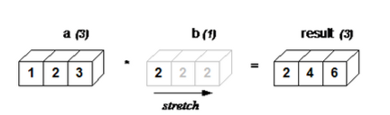
Broadcasting is a powerful mechanism that allows numpy to work with arrays of different shapes when performing arithmetic operations. Frequently we have a smaller array and a larger array, and we want to use the smaller array multiple times to perform some operation on the larger array.

# We will add the vector v to each row of the matrix x,
# storing the result in the matrix y
x = np.array([[1,2,3], [4,5,6], [7,8,9], [10, 11, 12]])
v = np.array([1, 0, 1])
y = np.empty_like(x)   # Create an empty matrix with the same shape as x

# Add the vector v to each row of the matrix x with an explicit loop
for i in range(4):
    y[i, :] = x[i, :] + v

# Now y is the following
# [[ 2  2  4]
#  [ 5  5  7]
#  [ 8  8 10]
#  [11 11 13]]
print(y)

This works; however when the matrix x is very large, computing an explicit loop in Python could be slow. Note that adding the vector v to each row of the matrix x  is equivalent to forming a matrix vv by stacking multiple copies of v  vertically, then performing elementwise summation of x and vv .

# We will add the vector v to each row of the matrix x,
# storing the result in the matrix y
x = np.array([[1,2,3], [4,5,6], [7,8,9], [10, 11, 12]])
v = np.array([1, 0, 1])
vv = np.tile(v, (4, 1))   # Stack 4 copies of v on top of each other
print(vv)                 # Prints "[[1 0 1]
                          #          [1 0 1]
                          #          [1 0 1]
                          #          [1 0 1]]"
y = x + vv  # Add x and vv elementwise
print(y)  # Prints "[[ 2  2  4
          #          [ 5  5  7]
          #          [ 8  8 10]
          #          [11 11 13]]"

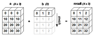
The line `y = x + v` works even though x has shape (4, 3) and v has shape (3,) due to broadcasting; this line works as if v actually had shape (4, 3), where each row was a copy of v, and the sum was performed elementwise.

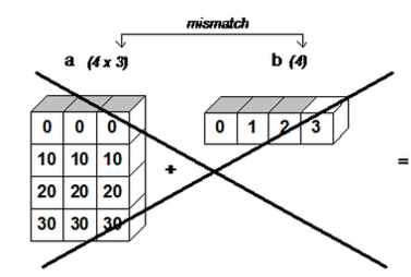
Broadcasting two arrays together follows these rules:

1. If the arrays do not have the same rank, prepend the shape of the lower rank array with 1s until both shapes have the same length.
2. The two arrays are said to be compatible in a dimension if they have the same size in the dimension, or if one of the arrays has size 1 in that dimension.
3. The arrays can be broadcast together if they are compatible in all dimensions.
4. After broadcasting, each array behaves as if it had shape equal to the elementwise maximum of shapes of the two input arrays.
5. In any dimension where one array had size 1 and the other array had size greater than 1, the first array behaves as if it were copied along that dimension

# Example applications of broadcasting

# Compute outer product of vectors
v = np.array([1,2,3])  # v has shape (3,)
w = np.array([4,5])    # w has shape (2,)

# To compute an outer product, we first reshape v to be a column
# vector of shape (3, 1); we can then broadcast it against w to yield
# an output of shape (3, 2), which is the outer product of v and w:
# [[ 4  5]
#  [ 8 10]
#  [12 15]]
print(np.reshape(v, (3, 1)) * w)

# Add a vector to each row of a matrix
x = np.array([[1,2,3], [4,5,6]])
# x has shape (2, 3) and v has shape (3,) so they broadcast to (2, 3),
# giving the following matrix:
# [[2 4 6]
#  [5 7 9]]
print(x + v)

# Add a vector to each column of a matrix
# x has shape (2, 3) and w has shape (2,).
# If we transpose x then it has shape (3, 2) and can be broadcast
# against w to yield a result of shape (3, 2); transposing this result
# yields the final result of shape (2, 3) which is the matrix x with
# the vector w added to each column. Gives the following matrix:
# [[ 5  6  7]
#  [ 9 10 11]]
print((x.T + w).T)
# Another solution is to reshape w to be a column vector of shape (2, 1);
# we can then broadcast it directly against x to produce the same
# output.
print(x + np.reshape(w, (2, 1)))

# Multiply a matrix by a constant:
# x has shape (2, 3). Numpy treats scalars as arrays of shape ();
# these can be broadcast together to shape (2, 3), producing the
# following array:
# [[ 2  4  6]
#  [ 8 10 12]]
print(x * 2)

---

💡 브로드캐스팅(Broadcasting)

Numpy에서 말하는 Broadcasting은 일정 조건을 부합하는 다른 형태의 배열끼리 연산을 수행하는 것을 의미한다.
즉, Numpy가 연산 중에 다른 모양(shapes)의 배열을 처리하는 방법을 설명한다. 더 작은 배열은 더 큰 배열에 ‘브로드캐스트’되어 호환되는 모양을 가진다.

import numpy as np
 
Value = np.array([[2,10,15],[1,2,3]])
 
Value1 = np.array([1])
 
Value2 = np.array([1,2])
 
print(Value + Value1)
 
print(Value + Value2)

# Results
# [[ 3 11 16] 
#  [ 2  3  4]]
 
# Traceback (most recent call last):
#  
#   File "C:/Users/Bens/PycharmProjects/Blogger/ndarrayma.py", line 8, in <module>
#  
#     print(Value + Value2)
#     
# ValueError: operands could not be broadcast together with shapes (2,3) (2,)

---

👉브로드캐스팅의 조건

1. 멤버가 하나인 배열은 어떤 배열에나 브로드캐스팅(Broadcasting)이 가능
   1. (단, 맴버가 하나도 없는 빈 배열을 제외) ex) 4x4 + 1

 

1. 하나의 배열의 차원이 1인 경우 브로드캐스팅(Broadcasting)이 가능 ex) 4x4 + 1x4

1. 차원의 짝이 맞을 때 브로드캐스팅(Broadcasting)가능
2. ex) 3x1 + 1x3

import numpy as np
 
Value = np.array([[1,2,3,4],[2,5,6,7],[8,9,10,11],[12,13,14,15]])
 
Value1 = np.array([1])
 
Value2 = np.array([3,3,3,3])
 
Value3 = np.array([4,5,6,7]).reshape(4,1)
 
print(Value + Value1) #4x4 + 1
 
print(Value + Value2) #4x4 + 1x4
 
print(Value2 + Value3) #1x4 + 4x1

# =============================================================================
# result for print(Value + Value1), 4x4 + 1
 
# [[ 2  3  4  5]
#  
#  [ 3  6  7  8]
#  
#  [ 9 10 11 12]
#  
#  [13 14 15 16]]
 
# result for print(Value + Value1), 4x4 + 1x4
 
# [[ 4  5  6  7]
#  
#  [ 5  8  9 10]
#  
#  [11 12 13 14]
#  
#  [15 16 17 18]]
 
# result for print(Value + Value1), 4x1 + 1x4
 
# [[ 7  7  7  7]
#  
#  [ 8  8  8  8]
#  
#  [ 9  9  9  9]
#  
#  [10 10 10 10]]

# Module Import
import numpy as np

Boolean array indexing

Boolean array indexing lets you pick out arbitrary elements of an array. Frequently this type of indexing is used to select the elements of an array that satisfy some condition.

a = np.array([1,2],[3,4],[5,6])
bool_idx = (a > 2) # Find the elements of a that are bigger than 2
									 # this returns a numpy array of Booleans of the same
									 # shape as a, where each slot of bool_idx tells
									 # whether that element of a in > 2.
print(bool_idx)
# [[False False],
#  [True   True],
#  [True   True]]

# We use boolean array indexing to construct a rank 1 array
# consisting of the elements of a corresponding to the True values
# of bool_idx
print(a[bool_idx]) # [3,4,5,6]

# We can do all of the above in a single concise statement:
print(a[a>2]) # [3,4,5,6]

Datatypes

Every numpy array is a grid of elements of the same type. Numpy provides a large set of numeric datatypes that you can use to construct arrays. Numpy tries to guess a datatype when you create an array, but functions that construct arrays usually also include an optional argument to explicitly specify the datatype.

x = np.array([1,2])
print(x.dtype) # int64

x = np.array([1.0, 2.0])
print(x.dtype) # float64

x = np.array([1,2], dtype=np.int64)
print(x.dtype) # int64

Array math

Basic mathematical functions operate elementwise on arrays, and are available both as operator overloads and as functions in the numpy module

x = np.array([[1,2],[3,4]], dtype=np.float64)
y = np.array([[5,6],[7,8]], dtype=np.float64)

# Elementwise sum; both produce the array
# [[ 6.0  8.0]
#  [10.0 12.0]]
print(x + y)
print(np.add(x, y))

# Elementwise difference; both produce the array
# [[-4.0 -4.0]
#  [-4.0 -4.0]]
print(x - y)
print(np.subtract(x, y))

# Elementwise product; both produce the array
# [[ 5.0 12.0]
#  [21.0 32.0]]
print(x * y)
print(np.multiply(x, y))

# Elementwise division; both produce the array
# [[ 0.2         0.33333333]
#  [ 0.42857143  0.5       ]]
print(x / y)
print(np.divide(x, y))

# Elementwise square root; produces the array
# [[ 1.          1.41421356]
#  [ 1.73205081  2.        ]]
print(np.sqrt(x))

*is elementwise multiplication, not matrix multiplication. We instead use the ***dot function to compute inner products of vectors***, to multiply a vector by a matrix, and to multiply matrices. dot is available both as a function in the numpy module and as an instance method of array objects

x = np.array([[1,2],[3,4]])
y = np.array([[5,6],[7,8]])

v = np.array([9,10])
w = np.array([11, 12])

# Inner product of vectors; both produce 219
print(v.dot(w))
print(np.dot(v, w))

# Matrix / vector product; both produce the rank 1 array [29 67]
print(x.dot(v))
print(np.dot(x, v))

# Matrix / matrix product; both produce the rank 2 array
# [[19 22]
#  [43 50]]
print(x.dot(y))
print(np.dot(x, y))

Numpy provides many useful funtions for performing computations on arrays; one of the most useful is sum

x = np.array([[1,2],[3,4]])

print(np.sum(x))  # Compute sum of all elements; prints "10"
print(np.sum(x, axis=0))  # Compute sum of each column; prints "[4 6]"
print(np.sum(x, axis=1))  # Compute sum of each row; prints "[3 7]"

Apart from computing mathematical functions using arrays, we frequently need to reshape or otherwise manipulate data in arrays. The simplest example of this type of operation is transposing a matrix; to transpose a matrix, simply use the T attribute of an array object:

x = np.array([[1,2], [3,4]])
print(x)    # Prints "[[1 2]
            #          [3 4]]"
print(x.T)  # Prints "[[1 3]
            #          [2 4]]"

# Note that taking the transpose of a rank 1 array does nothing:
v = np.array([1,2,3])
print(v)    # Prints "[1 2 3]"
print(v.T)  # Prints "[1 2 3]"

Broadcasting

Broadcasting is a powerful mechanism that allows numpy to work with arrays of different shapes when performing arithmetic operations. Frequently we have a smaller array and a larger array, and we want to use the smaller array multiple times to perform some operation on the larger array.

# We will add the vector v to each row of the matrix x,
# storing the result in the matrix y
x = np.array([[1,2,3], [4,5,6], [7,8,9], [10, 11, 12]])
v = np.array([1, 0, 1])
y = np.empty_like(x)   # Create an empty matrix with the same shape as x

# Add the vector v to each row of the matrix x with an explicit loop
for i in range(4):
    y[i, :] = x[i, :] + v

# Now y is the following
# [[ 2  2  4]
#  [ 5  5  7]
#  [ 8  8 10]
#  [11 11 13]]
print(y)

This works; however when the matrix x is very large, computing an explicit loop in Python could be slow. Note that adding the vector v to each row of the matrix x  is equivalent to forming a matrix vv by stacking multiple copies of v  vertically, then performing elementwise summation of x and vv .

# We will add the vector v to each row of the matrix x,
# storing the result in the matrix y
x = np.array([[1,2,3], [4,5,6], [7,8,9], [10, 11, 12]])
v = np.array([1, 0, 1])
vv = np.tile(v, (4, 1))   # Stack 4 copies of v on top of each other
print(vv)                 # Prints "[[1 0 1]
                          #          [1 0 1]
                          #          [1 0 1]
                          #          [1 0 1]]"
y = x + vv  # Add x and vv elementwise
print(y)  # Prints "[[ 2  2  4
          #          [ 5  5  7]
          #          [ 8  8 10]
          #          [11 11 13]]"

The line y = x + v works even though x has shape (4, 3) and v has shape (3,) due to broadcasting; this line works as if v actually had shape (4, 3), where each row was a copy of v, and the sum was performed elementwise.

Broadcasting two arrays together follows these rules:

1. If the arrays do not have the same rank, prepend the shape of the lower rank array with 1s until both shapes have the same length.
2. The two arrays are said to be compatible in a dimension if they have the same size in the dimension, or if one of the arrays has size 1 in that dimension.
3. The arrays can be broadcast together if they are compatible in all dimensions.
4. After broadcasting, each array behaves as if it had shape equal to the elementwise maximum of shapes of the two input arrays.
5. In any dimension where one array had size 1 and the other array had size greater than 1, the first array behaves as if it were copied along that dimension

# Example applications of broadcasting

# Compute outer product of vectors
v = np.array([1,2,3])  # v has shape (3,)
w = np.array([4,5])    # w has shape (2,)

# To compute an outer product, we first reshape v to be a column
# vector of shape (3, 1); we can then broadcast it against w to yield
# an output of shape (3, 2), which is the outer product of v and w:
# [[ 4  5]
#  [ 8 10]
#  [12 15]]
print(np.reshape(v, (3, 1)) * w)

# Add a vector to each row of a matrix
x = np.array([[1,2,3], [4,5,6]])
# x has shape (2, 3) and v has shape (3,) so they broadcast to (2, 3),
# giving the following matrix:
# [[2 4 6]
#  [5 7 9]]
print(x + v)

# Add a vector to each column of a matrix
# x has shape (2, 3) and w has shape (2,).
# If we transpose x then it has shape (3, 2) and can be broadcast
# against w to yield a result of shape (3, 2); transposing this result
# yields the final result of shape (2, 3) which is the matrix x with
# the vector w added to each column. Gives the following matrix:
# [[ 5  6  7]
#  [ 9 10 11]]
print((x.T + w).T)
# Another solution is to reshape w to be a column vector of shape (2, 1);
# we can then broadcast it directly against x to produce the same
# output.
print(x + np.reshape(w, (2, 1)))

# Multiply a matrix by a constant:
# x has shape (2, 3). Numpy treats scalars as arrays of shape ();
# these can be broadcast together to shape (2, 3), producing the
# following array:
# [[ 2  4  6]
#  [ 8 10 12]]
print(x * 2)

💡 브로드캐스팅(Broadcasting)

Numpy에서 말하는 Broadcasting은 일정 조건을 부합하는 다른 형태의 배열끼리 연산을 수행하는 것을 의미한다. 즉, Numpy가 연산 중에 다른 모양(shapes)의 배열을 처리하는 방법을 설명한다. 더 작은 배열은 더 큰 배열에 ‘브로드캐스트’되어 호환되는 모양을 가진다.

import numpy as np
 
Value = np.array([[2,10,15],[1,2,3]])
 
Value1 = np.array([1])
 
Value2 = np.array([1,2])
 
print(Value + Value1)
 
print(Value + Value2)

# Results
# [[ 3 11 16] 
#  [ 2  3  4]]
 
# Traceback (most recent call last):
#  
#   File "C:/Users/Bens/PycharmProjects/Blogger/ndarrayma.py", line 8, in <module>
#  
#     print(Value + Value2)
#     
# ValueError: operands could not be broadcast together with shapes (2,3) (2,)

---

👉브로드캐스팅의 조건

1. 멤버가 하나인 배열은 어떤 배열에나 브로드캐스팅(Broadcasting)이 가능
2. (단, 맴버가 하나도 없는 빈 배열을 제외) ex) 4x4 + 1
3. 하나의 배열의 차원이 1인 경우 브로드캐스팅(Broadcasting)이 가능 ex) 4x4 + 1x4
4. 
5. 차원의 짝이 맞을 때 브로드캐스팅(Broadcasting)가능
6. ex) 3x1 + 1x3

import numpy as np
 
Value = np.array([[1,2,3,4],[2,5,6,7],[8,9,10,11],[12,13,14,15]])
 
Value1 = np.array([1])
 
Value2 = np.array([3,3,3,3])
 
Value3 = np.array([4,5,6,7]).reshape(4,1)
 
print(Value + Value1) #4x4 + 1
 
print(Value + Value2) #4x4 + 1x4
 
print(Value2 + Value3) #1x4 + 4x1

# =============================================================================
# result for print(Value + Value1), 4x4 + 1
 
# [[ 2  3  4  5]
#  
#  [ 3  6  7  8]
#  
#  [ 9 10 11 12]
#  
#  [13 14 15 16]]
 
# result for print(Value + Value1), 4x4 + 1x4
 
# [[ 4  5  6  7]
#  
#  [ 5  8  9 10]
#  
#  [11 12 13 14]
#  
#  [15 16 17 18]]
 
# result for print(Value + Value1), 4x1 + 1x4
 
# [[ 7  7  7  7]
#  
#  [ 8  8  8  8]
#  
#  [ 9  9  9  9]
#  
#  [10 10 10 10]]

# Module Import
import numpy as np

Boolean array indexing

Boolean array indexing lets you pick out arbitrary elements of an array. Frequently this type of indexing is used to select the elements of an array that satisfy some condition.

a = np.array([1,2],[3,4],[5,6])
bool_idx = (a > 2) # Find the elements of a that are bigger than 2
									 # this returns a numpy array of Booleans of the same
									 # shape as a, where each slot of bool_idx tells
									 # whether that element of a in > 2.
print(bool_idx)
# [[False False],
#  [True   True],
#  [True   True]]

# We use boolean array indexing to construct a rank 1 array
# consisting of the elements of a corresponding to the True values
# of bool_idx
print(a[bool_idx]) # [3,4,5,6]

# We can do all of the above in a single concise statement:
print(a[a>2]) # [3,4,5,6]

Datatypes

Every numpy array is a grid of elements of the same type. Numpy provides a large set of numeric datatypes that you can use to construct arrays. Numpy tries to guess a datatype when you create an array, but functions that construct arrays usually also include an optional argument to explicitly specify the datatype.

x = np.array([1,2])
print(x.dtype) # int64

x = np.array([1.0, 2.0])
print(x.dtype) # float64

x = np.array([1,2], dtype=np.int64)
print(x.dtype) # int64

Array math

Basic mathematical functions operate elementwise on arrays, and are available both as operator overloads and as functions in the numpy module

x = np.array([[1,2],[3,4]], dtype=np.float64)
y = np.array([[5,6],[7,8]], dtype=np.float64)

# Elementwise sum; both produce the array
# [[ 6.0  8.0]
#  [10.0 12.0]]
print(x + y)
print(np.add(x, y))

# Elementwise difference; both produce the array
# [[-4.0 -4.0]
#  [-4.0 -4.0]]
print(x - y)
print(np.subtract(x, y))

# Elementwise product; both produce the array
# [[ 5.0 12.0]
#  [21.0 32.0]]
print(x * y)
print(np.multiply(x, y))

# Elementwise division; both produce the array
# [[ 0.2         0.33333333]
#  [ 0.42857143  0.5       ]]
print(x / y)
print(np.divide(x, y))

# Elementwise square root; produces the array
# [[ 1.          1.41421356]
#  [ 1.73205081  2.        ]]
print(np.sqrt(x))

*is elementwise multiplication, not matrix multiplication. We instead use the ***dot function to compute inner products of vectors***, to multiply a vector by a matrix, and to multiply matrices. dot is available both as a function in the numpy module and as an instance method of array objects

x = np.array([[1,2],[3,4]])
y = np.array([[5,6],[7,8]])

v = np.array([9,10])
w = np.array([11, 12])

# Inner product of vectors; both produce 219
print(v.dot(w))
print(np.dot(v, w))

# Matrix / vector product; both produce the rank 1 array [29 67]
print(x.dot(v))
print(np.dot(x, v))

# Matrix / matrix product; both produce the rank 2 array
# [[19 22]
#  [43 50]]
print(x.dot(y))
print(np.dot(x, y))

Numpy provides many useful funtions for performing computations on arrays; one of the most useful is sum

x = np.array([[1,2],[3,4]])

print(np.sum(x))  # Compute sum of all elements; prints "10"
print(np.sum(x, axis=0))  # Compute sum of each column; prints "[4 6]"
print(np.sum(x, axis=1))  # Compute sum of each row; prints "[3 7]"

Apart from computing mathematical functions using arrays, we frequently need to reshape or otherwise manipulate data in arrays. The simplest example of this type of operation is transposing a matrix; to transpose a matrix, simply use the T attribute of an array object:

x = np.array([[1,2], [3,4]])
print(x)    # Prints "[[1 2]
            #          [3 4]]"
print(x.T)  # Prints "[[1 3]
            #          [2 4]]"

# Note that taking the transpose of a rank 1 array does nothing:
v = np.array([1,2,3])
print(v)    # Prints "[1 2 3]"
print(v.T)  # Prints "[1 2 3]"

Broadcasting

Broadcasting is a powerful mechanism that allows numpy to work with arrays of different shapes when performing arithmetic operations. Frequently we have a smaller array and a larger array, and we want to use the smaller array multiple times to perform some operation on the larger array.

# We will add the vector v to each row of the matrix x,
# storing the result in the matrix y
x = np.array([[1,2,3], [4,5,6], [7,8,9], [10, 11, 12]])
v = np.array([1, 0, 1])
y = np.empty_like(x)   # Create an empty matrix with the same shape as x

# Add the vector v to each row of the matrix x with an explicit loop
for i in range(4):
    y[i, :] = x[i, :] + v

# Now y is the following
# [[ 2  2  4]
#  [ 5  5  7]
#  [ 8  8 10]
#  [11 11 13]]
print(y)

This works; however when the matrix x is very large, computing an explicit loop in Python could be slow. Note that adding the vector v to each row of the matrix x  is equivalent to forming a matrix vv by stacking multiple copies of v  vertically, then performing elementwise summation of x and vv .

# We will add the vector v to each row of the matrix x,
# storing the result in the matrix y
x = np.array([[1,2,3], [4,5,6], [7,8,9], [10, 11, 12]])
v = np.array([1, 0, 1])
vv = np.tile(v, (4, 1))   # Stack 4 copies of v on top of each other
print(vv)                 # Prints "[[1 0 1]
                          #          [1 0 1]
                          #          [1 0 1]
                          #          [1 0 1]]"
y = x + vv  # Add x and vv elementwise
print(y)  # Prints "[[ 2  2  4
          #          [ 5  5  7]
          #          [ 8  8 10]
          #          [11 11 13]]"

The line y = x + v works even though x has shape (4, 3) and v has shape (3,) due to broadcasting; this line works as if v actually had shape (4, 3), where each row was a copy of v, and the sum was performed elementwise.

Broadcasting two arrays together follows these rules:

1. If the arrays do not have the same rank, prepend the shape of the lower rank array with 1s until both shapes have the same length.
2. The two arrays are said to be compatible in a dimension if they have the same size in the dimension, or if one of the arrays has size 1 in that dimension.
3. The arrays can be broadcast together if they are compatible in all dimensions.
4. After broadcasting, each array behaves as if it had shape equal to the elementwise maximum of shapes of the two input arrays.
5. In any dimension where one array had size 1 and the other array had size greater than 1, the first array behaves as if it were copied along that dimension

# Example applications of broadcasting

# Compute outer product of vectors
v = np.array([1,2,3])  # v has shape (3,)
w = np.array([4,5])    # w has shape (2,)

# To compute an outer product, we first reshape v to be a column
# vector of shape (3, 1); we can then broadcast it against w to yield
# an output of shape (3, 2), which is the outer product of v and w:
# [[ 4  5]
#  [ 8 10]
#  [12 15]]
print(np.reshape(v, (3, 1)) * w)

# Add a vector to each row of a matrix
x = np.array([[1,2,3], [4,5,6]])
# x has shape (2, 3) and v has shape (3,) so they broadcast to (2, 3),
# giving the following matrix:
# [[2 4 6]
#  [5 7 9]]
print(x + v)

# Add a vector to each column of a matrix
# x has shape (2, 3) and w has shape (2,).
# If we transpose x then it has shape (3, 2) and can be broadcast
# against w to yield a result of shape (3, 2); transposing this result
# yields the final result of shape (2, 3) which is the matrix x with
# the vector w added to each column. Gives the following matrix:
# [[ 5  6  7]
#  [ 9 10 11]]
print((x.T + w).T)
# Another solution is to reshape w to be a column vector of shape (2, 1);
# we can then broadcast it directly against x to produce the same
# output.
print(x + np.reshape(w, (2, 1)))

# Multiply a matrix by a constant:
# x has shape (2, 3). Numpy treats scalars as arrays of shape ();
# these can be broadcast together to shape (2, 3), producing the
# following array:
# [[ 2  4  6]
#  [ 8 10 12]]
print(x * 2)

💡 브로드캐스팅(Broadcasting)

Numpy에서 말하는 Broadcasting은 일정 조건을 부합하는 다른 형태의 배열끼리 연산을 수행하는 것을 의미한다. 즉, Numpy가 연산 중에 다른 모양(shapes)의 배열을 처리하는 방법을 설명한다. 더 작은 배열은 더 큰 배열에 ‘브로드캐스트’되어 호환되는 모양을 가진다.

import numpy as np
 
Value = np.array([[2,10,15],[1,2,3]])
 
Value1 = np.array([1])
 
Value2 = np.array([1,2])
 
print(Value + Value1)
 
print(Value + Value2)

# Results
# [[ 3 11 16] 
#  [ 2  3  4]]
 
# Traceback (most recent call last):
#  
#   File "C:/Users/Bens/PycharmProjects/Blogger/ndarrayma.py", line 8, in <module>
#  
#     print(Value + Value2)
#     
# ValueError: operands could not be broadcast together with shapes (2,3) (2,)

---

👉브로드캐스팅의 조건

1. 멤버가 하나인 배열은 어떤 배열에나 브로드캐스팅(Broadcasting)이 가능
2. (단, 맴버가 하나도 없는 빈 배열을 제외) ex) 4x4 + 1
3. 하나의 배열의 차원이 1인 경우 브로드캐스팅(Broadcasting)이 가능 ex) 4x4 + 1x4
4. 
5. 차원의 짝이 맞을 때 브로드캐스팅(Broadcasting)가능
6. ex) 3x1 + 1x3

import numpy as np
 
Value = np.array([[1,2,3,4],[2,5,6,7],[8,9,10,11],[12,13,14,15]])
 
Value1 = np.array([1])
 
Value2 = np.array([3,3,3,3])
 
Value3 = np.array([4,5,6,7]).reshape(4,1)
 
print(Value + Value1) #4x4 + 1
 
print(Value + Value2) #4x4 + 1x4
 
print(Value2 + Value3) #1x4 + 4x1

# =============================================================================
# result for print(Value + Value1), 4x4 + 1
 
# [[ 2  3  4  5]
#  
#  [ 3  6  7  8]
#  
#  [ 9 10 11 12]
#  
#  [13 14 15 16]]
 
# result for print(Value + Value1), 4x4 + 1x4
 
# [[ 4  5  6  7]
#  
#  [ 5  8  9 10]
#  
#  [11 12 13 14]
#  
#  [15 16 17 18]]
 
# result for print(Value + Value1), 4x1 + 1x4
 
# [[ 7  7  7  7]
#  
#  [ 8  8  8  8]
#  
#  [ 9  9  9  9]
#  
#  [10 10 10 10]]

# Module Import
import numpy as np

Boolean array indexing

Boolean array indexing lets you pick out arbitrary elements of an array. Frequently this type of indexing is used to select the elements of an array that satisfy some condition.

a = np.array([1,2],[3,4],[5,6])
bool_idx = (a > 2) # Find the elements of a that are bigger than 2
									 # this returns a numpy array of Booleans of the same
									 # shape as a, where each slot of bool_idx tells
									 # whether that element of a in > 2.
print(bool_idx)
# [[False False],
#  [True   True],
#  [True   True]]

# We use boolean array indexing to construct a rank 1 array
# consisting of the elements of a corresponding to the True values
# of bool_idx
print(a[bool_idx]) # [3,4,5,6]

# We can do all of the above in a single concise statement:
print(a[a>2]) # [3,4,5,6]

Datatypes

Every numpy array is a grid of elements of the same type. Numpy provides a large set of numeric datatypes that you can use to construct arrays. Numpy tries to guess a datatype when you create an array, but functions that construct arrays usually also include an optional argument to explicitly specify the datatype.

x = np.array([1,2])
print(x.dtype) # int64

x = np.array([1.0, 2.0])
print(x.dtype) # float64

x = np.array([1,2], dtype=np.int64)
print(x.dtype) # int64

Array math

Basic mathematical functions operate elementwise on arrays, and are available both as operator overloads and as functions in the numpy module

x = np.array([[1,2],[3,4]], dtype=np.float64)
y = np.array([[5,6],[7,8]], dtype=np.float64)

# Elementwise sum; both produce the array
# [[ 6.0  8.0]
#  [10.0 12.0]]
print(x + y)
print(np.add(x, y))

# Elementwise difference; both produce the array
# [[-4.0 -4.0]
#  [-4.0 -4.0]]
print(x - y)
print(np.subtract(x, y))

# Elementwise product; both produce the array
# [[ 5.0 12.0]
#  [21.0 32.0]]
print(x * y)
print(np.multiply(x, y))

# Elementwise division; both produce the array
# [[ 0.2         0.33333333]
#  [ 0.42857143  0.5       ]]
print(x / y)
print(np.divide(x, y))

# Elementwise square root; produces the array
# [[ 1.          1.41421356]
#  [ 1.73205081  2.        ]]
print(np.sqrt(x))

*is elementwise multiplication, not matrix multiplication. We instead use the ***dot function to compute inner products of vectors***, to multiply a vector by a matrix, and to multiply matrices. dot is available both as a function in the numpy module and as an instance method of array objects

x = np.array([[1,2],[3,4]])
y = np.array([[5,6],[7,8]])

v = np.array([9,10])
w = np.array([11, 12])

# Inner product of vectors; both produce 219
print(v.dot(w))
print(np.dot(v, w))

# Matrix / vector product; both produce the rank 1 array [29 67]
print(x.dot(v))
print(np.dot(x, v))

# Matrix / matrix product; both produce the rank 2 array
# [[19 22]
#  [43 50]]
print(x.dot(y))
print(np.dot(x, y))

Numpy provides many useful funtions for performing computations on arrays; one of the most useful is sum

x = np.array([[1,2],[3,4]])

print(np.sum(x))  # Compute sum of all elements; prints "10"
print(np.sum(x, axis=0))  # Compute sum of each column; prints "[4 6]"
print(np.sum(x, axis=1))  # Compute sum of each row; prints "[3 7]"

Apart from computing mathematical functions using arrays, we frequently need to reshape or otherwise manipulate data in arrays. The simplest example of this type of operation is transposing a matrix; to transpose a matrix, simply use the T attribute of an array object:

x = np.array([[1,2], [3,4]])
print(x)    # Prints "[[1 2]
            #          [3 4]]"
print(x.T)  # Prints "[[1 3]
            #          [2 4]]"

# Note that taking the transpose of a rank 1 array does nothing:
v = np.array([1,2,3])
print(v)    # Prints "[1 2 3]"
print(v.T)  # Prints "[1 2 3]"

Broadcasting

Broadcasting is a powerful mechanism that allows numpy to work with arrays of different shapes when performing arithmetic operations. Frequently we have a smaller array and a larger array, and we want to use the smaller array multiple times to perform some operation on the larger array.

# We will add the vector v to each row of the matrix x,
# storing the result in the matrix y
x = np.array([[1,2,3], [4,5,6], [7,8,9], [10, 11, 12]])
v = np.array([1, 0, 1])
y = np.empty_like(x)   # Create an empty matrix with the same shape as x

# Add the vector v to each row of the matrix x with an explicit loop
for i in range(4):
    y[i, :] = x[i, :] + v

# Now y is the following
# [[ 2  2  4]
#  [ 5  5  7]
#  [ 8  8 10]
#  [11 11 13]]
print(y)

This works; however when the matrix x is very large, computing an explicit loop in Python could be slow. Note that adding the vector v to each row of the matrix x  is equivalent to forming a matrix vv by stacking multiple copies of v  vertically, then performing elementwise summation of x and vv .

# We will add the vector v to each row of the matrix x,
# storing the result in the matrix y
x = np.array([[1,2,3], [4,5,6], [7,8,9], [10, 11, 12]])
v = np.array([1, 0, 1])
vv = np.tile(v, (4, 1))   # Stack 4 copies of v on top of each other
print(vv)                 # Prints "[[1 0 1]
                          #          [1 0 1]
                          #          [1 0 1]
                          #          [1 0 1]]"
y = x + vv  # Add x and vv elementwise
print(y)  # Prints "[[ 2  2  4
          #          [ 5  5  7]
          #          [ 8  8 10]
          #          [11 11 13]]"

The line y = x + v works even though x has shape (4, 3) and v has shape (3,) due to broadcasting; this line works as if v actually had shape (4, 3), where each row was a copy of v, and the sum was performed elementwise.

Broadcasting two arrays together follows these rules:

1. If the arrays do not have the same rank, prepend the shape of the lower rank array with 1s until both shapes have the same length.
2. The two arrays are said to be compatible in a dimension if they have the same size in the dimension, or if one of the arrays has size 1 in that dimension.
3. The arrays can be broadcast together if they are compatible in all dimensions.
4. After broadcasting, each array behaves as if it had shape equal to the elementwise maximum of shapes of the two input arrays.
5. In any dimension where one array had size 1 and the other array had size greater than 1, the first array behaves as if it were copied along that dimension

# Example applications of broadcasting

# Compute outer product of vectors
v = np.array([1,2,3])  # v has shape (3,)
w = np.array([4,5])    # w has shape (2,)

# To compute an outer product, we first reshape v to be a column
# vector of shape (3, 1); we can then broadcast it against w to yield
# an output of shape (3, 2), which is the outer product of v and w:
# [[ 4  5]
#  [ 8 10]
#  [12 15]]
print(np.reshape(v, (3, 1)) * w)

# Add a vector to each row of a matrix
x = np.array([[1,2,3], [4,5,6]])
# x has shape (2, 3) and v has shape (3,) so they broadcast to (2, 3),
# giving the following matrix:
# [[2 4 6]
#  [5 7 9]]
print(x + v)

# Add a vector to each column of a matrix
# x has shape (2, 3) and w has shape (2,).
# If we transpose x then it has shape (3, 2) and can be broadcast
# against w to yield a result of shape (3, 2); transposing this result
# yields the final result of shape (2, 3) which is the matrix x with
# the vector w added to each column. Gives the following matrix:
# [[ 5  6  7]
#  [ 9 10 11]]
print((x.T + w).T)
# Another solution is to reshape w to be a column vector of shape (2, 1);
# we can then broadcast it directly against x to produce the same
# output.
print(x + np.reshape(w, (2, 1)))

# Multiply a matrix by a constant:
# x has shape (2, 3). Numpy treats scalars as arrays of shape ();
# these can be broadcast together to shape (2, 3), producing the
# following array:
# [[ 2  4  6]
#  [ 8 10 12]]
print(x * 2)

💡 브로드캐스팅(Broadcasting)

Numpy에서 말하는 Broadcasting은 일정 조건을 부합하는 다른 형태의 배열끼리 연산을 수행하는 것을 의미한다. 즉, Numpy가 연산 중에 다른 모양(shapes)의 배열을 처리하는 방법을 설명한다. 더 작은 배열은 더 큰 배열에 ‘브로드캐스트’되어 호환되는 모양을 가진다.

import numpy as np
 
Value = np.array([[2,10,15],[1,2,3]])
 
Value1 = np.array([1])
 
Value2 = np.array([1,2])
 
print(Value + Value1)
 
print(Value + Value2)

# Results
# [[ 3 11 16] 
#  [ 2  3  4]]
 
# Traceback (most recent call last):
#  
#   File "C:/Users/Bens/PycharmProjects/Blogger/ndarrayma.py", line 8, in <module>
#  
#     print(Value + Value2)
#     
# ValueError: operands could not be broadcast together with shapes (2,3) (2,)

---

👉브로드캐스팅의 조건

멤버가 하나인 배열은 어떤 배열에나 브로드캐스팅(Broadcasting)이 가능 (단, 맴버가 하나도 없는 빈 배열을 제외)
ex) 4x4 + 1

하나의 배열의 차원이 1인 경우 브로드캐스팅(Broadcasting)이 가능 ex) 4x4 + 1x4

차원의 짝이 맞을 때 브로드캐스팅(Broadcasting)가능  ex) 3x1 + 1x3

import numpy as np
 
Value = np.array([[1,2,3,4],[2,5,6,7],[8,9,10,11],[12,13,14,15]])
 
Value1 = np.array([1])
 
Value2 = np.array([3,3,3,3])
 
Value3 = np.array([4,5,6,7]).reshape(4,1)
 
print(Value + Value1) #4x4 + 1
 
print(Value + Value2) #4x4 + 1x4
 
print(Value2 + Value3) #1x4 + 4x1

# =============================================================================
# result for print(Value + Value1), 4x4 + 1
 
# [[ 2  3  4  5]
#  
#  [ 3  6  7  8]
#  
#  [ 9 10 11 12]
#  
#  [13 14 15 16]]
 
# result for print(Value + Value1), 4x4 + 1x4
 
# [[ 4  5  6  7]
#  
#  [ 5  8  9 10]
#  
#  [11 12 13 14]
#  
#  [15 16 17 18]]
 
# result for print(Value + Value1), 4x1 + 1x4
 
# [[ 7  7  7  7]
#  
#  [ 8  8  8  8]
#  
#  [ 9  9  9  9]
#  
#  [10 10 10 10]]